Les guides pour les nuls

Index

• OLS: ordinary LS
  • Formulation:
  • Solution:
• Flavors
  • WLS: Weighted LS
  • IRLS: Iteratively Reweighted LS
  • NLS: Nonlinear LS

OLS: ordinary LS

Formulation:

The standard formulation for a least-squares problem is given a system of linear equations

\[Ax = b\]

where $A \in \mathbf{R}^{m \times n}$, $x \in \mathbf{R}^n$, and $b \in \mathbf{R}^m$, solve the following minimization problem:

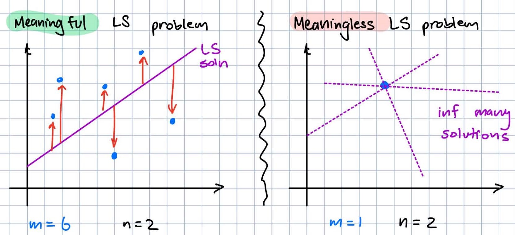
\[\argmin_{x} ||b - Ax||_2^{2}\]

It is important to note that $m>n$. If $m<n$, the minimization problem loses meaning. $m>n$ implies more equations (size of $b$) than unknowns (size of $x$). If we had more unknowns than equations ($m<n$) there is an infinite solution set.

Perhaps best driven home via the simplest sample of linear regression. In this figure, blue points are datapoints. Red indicates the LS errors. Recall that fitting any line on a 2d plane requires only the definition of a slope and a y-intcpt, which is why $n= 2$ unknowns is from.

Note on practicality: in fact, typically $m » n$ in engineering. If you are trying to say, solve for the unknown of your GPS location ($n \in \mathbf{R}^4$), you can have thousands of GPS satellite measurements within a minute ($m \in \mathbf{R}^{1000}$).

Solution:

At face value, the solution to the least-squares problem is

\[\boxed{x = (A^TA)^{-1}A^Tb}\]

Where $(A^TA)^{-1}A^T$ should look familiar as the left-pseudoinverse of $A$. This solution is best committed to memory.

A few notes

• We see again that if $m<n$, $A^TA$ would not be full rank, and hence we cannot take $(A^TA)^{-1}$; thus further solidifying the meaninglessness of LS with $m<n$
• Although the pseudoinverse can be arrived from very simple alg manipulation, why it works as a solution to the minimazation problem is not evident and merits a proof.
• for the curious, the right-pseudoinverse also exists for the dual of the Least-Squares problem: the Least-Norm problem (which seeks to minimize magnitude $x^Tx$ for the infinitely possible solns $x$.) perhaps one day this far less common problem finds its way into these notes.

Solution Derivation:

\[\begin{align*} &\argmin_{x} ||Ax - b||^2_2\\ \Rightarrow & \argmin_{x} (Ax - b)^T(Ax - b) \\ \Rightarrow & \argmin_{x} (x^TA^TAx - x^TA^Tb - b^TAx + b^Tb) \\ \end{align*}\]

From here we see the function we are minimizing over is quadratic in $x$. Additionally $A^TA$ is by definition always PSD regardless of $A$. Thus the function is also convex. This makes minimizing simple.

\[\begin{align*} \frac{\partial}{\partial x}(x^TA^TAx - x^TA^Tb - b^TAx + b^Tb) &= 0\\ \frac{\partial}{\partial x}(x^TA^TAx - 2x^TA^Tb + b^Tb) &= 0\\ 2A^TAx - 2A^T b &= 0\\ x & = (A^TA)^{-1}A^Tb \end{align*}\]

voila.

Flavors

WLS: Weighted LS

Weighted LS is a simple natural extension of OLS. The key difference is in the addition of a diagonal, square weight matrix $W$.

\[W \triangleq \begin{bmatrix} w_1 & \dots & 0 \\ \vdots & \ddots & \vdots \\ 0 & \dots & w_n \end{bmatrix}\]

Where every scalar weight $w_i$ is the weight placed on the $i$th residual.

We can intuitively infer that this is most practical when certain datapoints in the problem are “less trustworth” than others, meriting a lower weight. Following this philosophy, we see why each weight is defined as the inverse of the variance of the associated point.

\[w_i \triangleq \frac{1}{\sigma_i^2}\]

The OLS problem now becomes the WLS problem by simply scaling the objective function by $W$.

\[\argmin_{x} (Ax - b)^TW(Ax - b)\]

Solving as with the OLS yields $\boxed{x = (A^TWA)^{-1}A^TWb}$

IRLS: Iteratively Reweighted LS

IRLS is another extension of WLS, used often for sequential LS estimation problems, which is where the “iteration” is introduced.

NLS: Nonlinear LS

Returning to OLS, we can further extend OLS with NLS. In general, linearity is a very strong assumption to have for model fitting, but nonlinearity makes me cry. NLS is a numerical extension to the pure analytical solution of OLS. NLS iteratively linearizes around local datapoints and solves a small local OLS problem. This will be a very common theme in MANY algorithms modified for nonlinearity (EKF, LQR, etc…). note to self, jacobian linearization should definitely live elsewhere.